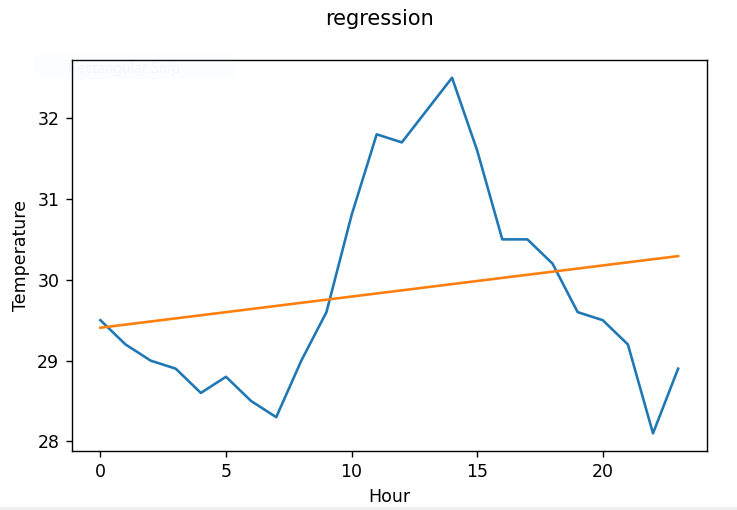
This article is to convert the implementation of the regression model from the article of ESP32-C3 to NumPy on Raspberry Pi and PC and use the display as Matplotlib, as shown in Figure 1, which can be found from the previous article. The temperature and humidity from the 1-day data were obtained from parameters a and b of the regression equation and the resulting equation or model was used to determine the possible temperature values over the 1 day.
Code
The program code adapted from the previous article is as follows.
import numpy as np
import matplotlib.pyplot as plt

n = 24
x = np.arange(n)
y = np.array([29.5, 29.2, 29.0, 28.9, 28.6, 28.8, 28.5, 28.3, 29.0, 29.6, 30.8, 31.8, 31.7, 32.1, 32.5, 31.6, 30.5, 30.5, 30.2, 29.6, 29.5, 29.2, 28.1, 28.9])

sumX = np.sum(x)
sumY = np.sum(y)
sumXY = np.sum(x*y)
sumX2= np.sum(x*x)
sumY2 = np.sum(y*y)

print("SumX={}".format(sumX))
print("SumY={}".format(sumY))
print("SumXY={}".format(sumXY))
print("SumX2={}".format(sumX2))
print("SumY2={}".format(sumY2))

a = ((sumY*sumX2)-(sumX*sumXY))/((n*sumX2)-(sumX*sumX))
b = ((n*sumXY)-(sumX*sumY))/((n*sumX2)-(sumX*sumX))
print("Y = ({})+({}*x)+c".format(a,b))

z = a+(b*x)
print(z)

plt.suptitle('regression')
plt.ylabel('Temperature')
plt.xlabel('Hour')
plt.subplot(111)
plt.plot(y)
plt.subplot(111)
plt.plot(z)
plt.show()
From the program, the work can be divided into 4 steps:
- Create variables x and y to store hour values and hourly temperature.
- Calculate the sum of x, y, x*y, x*x and y*y.
- Find the values of a and b.
- Rendered with matplotlib.
Create variables
From the ulab article on array and numpy, we can create data variables with numpy.array() and numpy.arange() for creating arrays. When creating a variable x holding the values 0 through 23, you may use the arange() statement to create the bottom row of data in a given range and create a variable y with array() specifying the values of each member as follows:
x = np.arange(n)
y = np.array([29.5, 29.2, 29.0, 28.9, 28.6, 28.8, 28.5, 28.3, 29.0, 29.6, 30.8, 31.8, 31.7, 32.1, 32.5, 31.6, 30.5, 30.5, 30.2, 29.6, 29.5, 29.2, 28.1, 28.9])
Calculate
The working principle of numpy applies computations to the entire dataset, so when a scalar is applied to a numpy-generated variable, it acts on every element within that variable. And the action between variables together will perform that action on members of the same order. The numpy.sum() command can be used to sum all members in a variable. Therefore, the code for summing x, y, x*y, x*x and y*y can be written as follows.
sumX = np.sum(x)
sumY = np.sum(y)
sumXY = np.sum(x*y)
sumX2= np.sum(x*x)
sumY2 = np.sum(y*y)
Find the values of a and b.
Calculating for a and b for the following linear equations
Y = a + bX + c
where
a=( (Σy)(Σx2) – (Σx)(Σxy) ) / ( n(Σx2) – (Σx)2)
b= (n (Σxy) – (Σx)(Σy) ) / (n(Σx2) – (Σx)2)
Code
a = ((sumY*sumX2)-(sumX*sumXY))/((n*sumX2)-(sumX*sumX))
b = ((n*sumXY)-(sumX*sumY))/((n*sumX2)-(sumX*sumX))
Render
When rendered with a graph via matplotlib, it can be written as follows: The result of the display is as shown in Figure 1.
plt.suptitle('regression')
plt.ylabel('Temperature')
plt.xlabel('Hour')
plt.subplot(111)
plt.plot(y)
plt.subplot(111)
plt.plot(z)
plt.show()
Conclusion
From this article, you will find that Python programming has the advantage of being cross-platform, making it possible to transfer code from esp32 to a Raspberry Pi or PC. With the graph rendering library matplotlib, programmers can display a wide range of applications and beautiful. Therefore, learning the library and choosing the library saves development time. And it’s suitable for making a prototype to improve the work further. Finally, have fun with programming.
(C) 2020-2022, By Jarut Busarathid and Danai Jedsadathitikul
Updated 2022-02-10